Data Manipulation with N-dimensional Arrays

Chapter 2.1: Preliminaries

Based on "Dive into Deep Learning" by Zhang et al.

Instructor: Guðmundur Einarsson
University of Iceland

Based on slides from Hafsteinn Einarsson

Learning Objectives

Understand tensorsA tensor is a generalization of vectors and matrices to potentially higher dimensions. In deep learning, tensors are the fundamental data structure for storing and manipulating data. and their role in deep learning
Master tensor creation and manipulation
Learn indexing, slicing, and reshaping operations
Understand broadcastingBroadcasting is a mechanism that allows operations on tensors of different shapes by automatically expanding dimensions to make them compatible. mechanism
Optimize memory usage in tensor operations
Convert between different data formats

What are Tensors?

A tensorA (possibly multidimensional) array of numerical values. The fundamental data structure in deep learning frameworks. represents an n-dimensional array of numerical values

0D tensor: Scalar (single number)
1D tensor: Vector
2D tensor: Matrix
3D+ tensor: Higher-order tensor

Tensors are the foundation of all deep learning computations!

Creating Tensors: arange()

Create a vector of evenly spaced values

import torch

# Create a tensor with values from 0 to 11
x = torch.arange(12, dtype=torch.float32)
print(x)

tensor([ 0.,  1.,  2.,  3.,  4.,  5.,  6.,  7.,  8.,  9., 10., 11.])

Each value is called an elementAn individual value within a tensor. Elements can be accessed and modified using indexing. of the tensor

Tensor Properties

Inspect tensor characteristics

# Number of elements
print(x.numel())  # 12

# Shape of the tensor
print(x.shape)     # torch.Size([12])

# Data type
print(x.dtype)     # torch.float32

Shape tells us the size along each dimension

Reshaping Tensors

Change shape without altering values

# Reshape vector to 3x4 matrix
X = x.reshape(3, 4)
print(X)

tensor([[ 0.,  1.,  2.,  3.],
        [ 4.,  5.,  6.,  7.],
        [ 8.,  9., 10., 11.]])

# Use -1 to infer dimension
X = x.reshape(-1, 4)  # Same as reshape(3, 4)
X = x.reshape(3, -1)  # Same as reshape(3, 4)

Creating Special Tensors

Initialize with specific values

# Tensor of zeros
zeros = torch.zeros((2, 3, 4))

# Tensor of ones  
ones = torch.ones((2, 3, 4))

# Random values from standard normal distribution
randn = torch.randn(3, 4)

# From Python list
tensor = torch.tensor([[2, 1, 4, 3],
                       [1, 2, 3, 4],
                       [4, 3, 2, 1]])

Test Your Understanding

Indexing and Slicing

Access and modify tensor elements

Similar to Python lists
Zero-based indexing
Negative indexing from end
Slicing with start:stop syntax

Basic Indexing

X = torch.arange(12).reshape(3, 4)

# Access last row
print(X[-1])
# tensor([8., 9., 10., 11.])

# Access rows 1 and 2
print(X[1:3])
# tensor([[4., 5., 6., 7.],
#         [8., 9., 10., 11.]])

Writing Elements

Modify tensor values by index

# Modify single element
X[1, 2] = 17
print(X)

tensor([[ 0.,  1.,  2.,  3.],
        [ 4.,  5., 17.,  7.],
        [ 8.,  9., 10., 11.]])

# Modify multiple elements
X[:2, :] = 12  # First two rows
print(X)

tensor([[12., 12., 12., 12.],
        [12., 12., 12., 12.],
        [ 8.,  9., 10., 11.]])

Test Your Understanding

Tensor Operations

Mathematical operations on tensors

Elementwise operations: Apply to each element
Unary operations: Single input (e.g., exp, log)
Binary operations: Two inputs (e.g., +, -, *, /)

Operations preserve tensor shape when inputs have same shape

Unary Operations

Operations on single tensors

x = torch.tensor([1.0, 2, 4, 8])

# Exponential function
print(torch.exp(x))
# tensor([2.7183e+00, 7.3891e+00, 5.4598e+01, 2.9810e+03])

Mathematical notation: f: ℝ → ℝA function that maps from any real number to another real number, applied elementwise to each tensor element.

Binary Operations

Operations on pairs of tensors

x = torch.tensor([1.0, 2, 4, 8])
y = torch.tensor([2, 2, 2, 2])

print(x + y)  # tensor([ 3.,  4.,  6., 10.])
print(x - y)  # tensor([-1.,  0.,  2.,  6.])
print(x * y)  # tensor([ 2.,  4.,  8., 16.])
print(x / y)  # tensor([0.5, 1.0, 2.0, 4.0])
print(x ** y) # tensor([ 1.,  4., 16., 64.])

Mathematical notation: f: ℝ, ℝ → ℝA function that takes two real numbers and returns a real number, applied elementwise to pairs of tensor elements.

Concatenation

Combine tensors along an axis

X = torch.arange(12, dtype=torch.float32).reshape((3,4))
Y = torch.tensor([[2.0, 1, 4, 3],
                  [1, 2, 3, 4],
                  [4, 3, 2, 1]])

# Concatenate along rows (axis 0)
Z1 = torch.cat((X, Y), dim=0)
print(Z1.shape)  # torch.Size([6, 4])

# Concatenate along columns (axis 1)
Z2 = torch.cat((X, Y), dim=1)
print(Z2.shape)  # torch.Size([3, 8])

Logical Operations

Element-wise comparisons

X = torch.arange(12).reshape(3, 4)
Y = X.clone()
Y[1, 2] = 6  # Same as X[1, 2]

print(X == Y)

tensor([[True, True, True, True],
        [True, True, True, True],
        [True, True, True, True]])

# Sum all elements
print(X.sum())  # tensor(66.)

Test Your Understanding

Broadcasting Mechanism

Operations on different-shaped tensors

BroadcastingA mechanism that automatically expands tensors to compatible shapes for element-wise operations without actually copying data. enables operations between tensors of different shapes

Two-step process:

Expand arrays by copying elements along axes with length 1
Perform element-wise operation on resulting arrays

Broadcasting Example

a = torch.arange(3).reshape((3, 1))
b = torch.arange(2).reshape((1, 2))

print("a:")
print(a)
print("\nb:")
print(b)

a:
tensor([[0],
        [1],
        [2]])

b:
tensor([[0, 1]])

Broadcasting Addition

# a is (3, 1), b is (1, 2)
# Broadcasting expands to (3, 2)
result = a + b
print(result)

tensor([[0, 1],
        [1, 2],
        [2, 3]])

Broadcasting conceptually replicates:
a → [[0, 0], [1, 1], [2, 2]]
b → [[0, 1], [0, 1], [0, 1]]

Broadcasting Rules

Two tensors are compatible for broadcasting if:

Their dimensions are equal, OR
One of them is 1, OR
One of them doesn't exist

# Examples of compatible shapes:
# (3, 1) and (1, 4) → (3, 4)
# (5, 3, 4) and (3, 4) → (5, 3, 4)
# (5, 3, 4) and (1, 4) → (5, 3, 4)
# (15, 3, 5) and (15, 1, 5) → (15, 3, 5)

Test Your Understanding

Memory Management

Efficient tensor operations

Operations can allocate new memory unnecessarily

before = id(Y)
Y = Y + X  # Creates new tensor
print(id(Y) == before)  # False

In ML, we update millions of parameters frequently - memory efficiency matters!

In-Place Operations

Modify tensors without allocating new memory

# Method 1: Slice notation
Z = torch.zeros_like(Y)
print('id(Z):', id(Z))
Z[:] = X + Y  # In-place assignment
print('id(Z):', id(Z))  # Same ID!

# Method 2: In-place operators
before = id(X)
X += Y  # Equivalent to X[:] = X + Y
print(id(X) == before)  # True

In-Place Operation Methods

PyTorch provides in-place method variants

# Operations ending with _ are in-place
X.add_(Y)     # X += Y
X.mul_(2)     # X *= 2
X.sub_(1)     # X -= 1
X.div_(2)     # X /= 2

# These modify X directly without new allocation

⚠️ Be careful: In-place operations can break gradient computation!

Test Your Understanding

Converting Between Formats

Interoperability with NumPy and Python

Convert to/from NumPy arrays
Extract Python scalars
Share memory (PyTorch) or copy (other frameworks)

NumPy Conversion

# PyTorch to NumPy
X = torch.ones(5)
A = X.numpy()
print(type(A))  # 

# NumPy to PyTorch
B = torch.from_numpy(A)
print(type(B))  #

⚠️ PyTorch CPU tensors share memory with NumPy arrays!

Converting to Python Scalars

# Single element tensor to scalar
a = torch.tensor([3.5])

# Method 1: item()
scalar1 = a.item()
print(scalar1)  # 3.5

# Method 2: Python built-ins
scalar2 = float(a)
print(scalar2)  # 3.5

scalar3 = int(a)
print(scalar3)  # 3

Only works for tensors with exactly one element!

Framework Comparison

Framework	Tensor Class	NumPy Sharing
PyTorch	Tensor	Shares memory (CPU)
TensorFlow	Tensor	Copies data
MXNet	ndarray	Copies data
JAX	Array	Copies data

Test Your Understanding

Data Processing

Preparing real-world data for deep learning

Raw data is rarely ready for machine learning

Missing values
Inconsistent formats
Categorical variables
Different scales

80% of data science is cleaning and preparing data!

pandas: Python Data Analysis Library

The standard tool for data manipulation in Python

Key Data Structures:

DataFrameA 2D labeled data structure with columns of potentially different types, like a spreadsheet or SQL table. - 2D table with labeled axes
SeriesA 1D labeled array capable of holding any data type. Each column in a DataFrame is a Series. - 1D labeled array

import pandas as pd
import numpy as np
import torch

Test Your Understanding

Reading Data from CSV

# Create a sample CSV file
import os
os.makedirs('data', exist_ok=True)
data_file = 'data/house_tiny.csv'

with open(data_file, 'w') as f:
    f.write('''NumRooms,RoofType,Price
NA,NA,127500
2,NA,106000
4,Slate,178100
NA,NA,140000''')

# Read the CSV file
data = pd.read_csv(data_file)
print(data)

Inspecting Data

# First few rows
print(data.head())
# Data types and non-null counts
print(data.info())
# Statistical summary
print(data.describe())
# Check for missing values
print(data.isna().sum())

   NumRooms RoofType    Price
0       NaN      NaN   127500
1       2.0      NaN   106000
2       4.0    Slate   178100
3       NaN      NaN   140000

Test Your Understanding

Handling Missing Data

Strategies for dealing with NaN values

Common Approaches:

Deletion: Remove rows/columns with missing values
Imputation: Fill with estimated values
Indicator: Create binary flag for missingness

It is good to try to know whether data is missing at random or whether we are dealing with structured missingness

How can data be missing in a systematic way?

Choice depends on data characteristics and problem requirements

Separating Features and Target

# Separate input features and target variable
inputs, targets = data.iloc[:, 0:2], data.iloc[:, 2]

print("Input features:")
print(inputs)
print("\nTarget values:")
print(targets)

Input features:
   NumRooms RoofType
0       NaN      NaN
1       2.0      NaN...
Target values:
0    127500
1    106000...

Numerical Imputation

# Fill NaN with mean for numerical columns
numeric_cols = inputs.select_dtypes(include=[np.number]).columns
inputs[numeric_cols] = inputs[numeric_cols].fillna(
    inputs[numeric_cols].mean()
)

print(inputs)

   NumRooms RoofType
0       3.0      NaN
1       2.0      NaN
2       4.0    Slate
3       3.0      NaN

Mean of [NaN, 2, 4, NaN] = 3.0

Categorical Imputation

# Convert categorical columns to dummy variables
# dummy_na=True creates indicator for NaN
inputs = pd.get_dummies(inputs, dummy_na=True)
print(inputs)

   NumRooms  RoofType_Slate  RoofType_nan
0       3.0               0             1
1       2.0               0             1
2       4.0               1             0
3       3.0               0             1

One-hot encoding converts categories to binary columns

Test Your Understanding

Data Selection and Filtering

Accessing specific parts of your data

Selection Methods:

.iloc[] - Integer position based
.loc[] - Label based
[] - Column selection
Boolean indexing - Conditional filtering

Selection Examples

# Create sample DataFrame
df = pd.DataFrame({
    'A': [1, 2, 3, 4],
    'B': [5, 6, 7, 8],
    'C': [9, 10, 11, 12]
})

# Select by position
print(df.iloc[0:2, 1:3])  # First 2 rows, columns 1-2

# Select by label
print(df.loc[:, ['A', 'C']])  # All rows, columns A and C

# Boolean indexing
print(df[df['A'] > 2])  # Rows where column A > 2

Feature Engineering

Creating new features from existing data

# Create new features
df['D'] = df['A'] + df['B']  # Sum of two columns
df['E'] = df['C'].apply(lambda x: x**2)  # Square values
df['F'] = (df['A'] > 2).astype(int)  # Binary feature

print(df.head())

Certain transformations are common, e.g., a log transform for very skewed values

Good features can dramatically improve model performance!

Test Your Understanding

Converting to Tensors

Preparing data for deep learning frameworks

Neural networks require numerical tensors as input

# Convert DataFrame to NumPy array
numpy_array = inputs.to_numpy(dtype=float)

# Convert to PyTorch tensor
X = torch.tensor(numpy_array, dtype=torch.float32)
y = torch.tensor(targets.to_numpy(dtype=float), 
                 dtype=torch.float32)

Complete Workflow Example

# 1. Load data
data = pd.read_csv('data/house_tiny.csv')

# 2. Split features and target
inputs, targets = data.iloc[:, :-1], data.iloc[:, -1]

# 3. Handle missing values
numeric_cols = inputs.select_dtypes(include=[np.number]).columns
inputs[numeric_cols] = inputs[numeric_cols].fillna(
    inputs[numeric_cols].mean()
)
inputs = pd.get_dummies(inputs, dummy_na=True)

# 4. Convert to tensors
X = torch.tensor(inputs.to_numpy(dtype=float), dtype=torch.float32)
y = torch.tensor(targets.to_numpy(dtype=float), dtype=torch.float32)

print(f"Features shape: {X.shape}")
print(f"Target shape: {y.shape}")

Data Processing Pipeline

Each step transforms data closer to ML-ready format

Test Your Understanding

Linear Algebra for Deep Learning

Mathematical foundations for neural networks

Learning Objectives:

Understand scalars, vectors, matrices, and tensors
Master fundamental operations (addition, multiplication)
Learn reduction operations and norms
Connect linear algebra to deep learning

Linear algebra is the language of deep learning!

Scalars

A scalarA single numerical value, as opposed to a vector or matrix. In deep learning, scalars often represent single measurements like loss or accuracy. is a single number

Denoted by lowercase letters: x, y, z
Can be integers or real numbers
Examples: temperature, price, count

import torch
# Create scalars
x = torch.tensor(3.0)
y = torch.tensor(2.0)
# Scalar operations
print(x + y)  # tensor(5.)
print(x * y)  # tensor(6.)
print(x / y)  # tensor(1.5)
print(x ** y) # tensor(9.)

Vectors

A vectorAn ordered array of scalars. In deep learning, vectors often represent features, weights, or activations for a single example. is an ordered list of scalar values

$$\mathbf{x} = \begin{bmatrix} x_1 \\ x_2 \\ \vdots \\ x_n \end{bmatrix}$$

# Create vectors
x = torch.arange(3, dtype=torch.float32)
print(x)  # tensor([0., 1., 2.])

# Access elements
print(x[0])  # tensor(0.)
print(len(x))  # 3
print(x.shape)  # torch.Size([3])

Vector Operations

Element-wise and special operations

u = torch.tensor([3.0, -4.0])
v = torch.tensor([2.0, 1.0])

# Element-wise operations
print(u + v)  # tensor([5., -3.])
print(u - v)  # tensor([1., -5.])
print(u * v)  # tensor([6., -4.])  # Hadamard product

# Scalar multiplication
alpha = 2
print(alpha * u)  # tensor([6., -8.])

Most vector operations are element-wise by default!

Test Your Understanding

Matrices

2D arrays of scalars

A matrixA 2D array of numbers arranged in rows and columns. In deep learning, matrices often represent weights, batches of vectors, or transformations. is a 2D array with m rows and n columns

$$\mathbf{A} = \begin{bmatrix} a_{11} & a_{12} & \cdots & a_{1n} \\ a_{21} & a_{22} & \cdots & a_{2n} \\ \vdots & \vdots & \ddots & \vdots \\ a_{m1} & a_{m2} & \cdots & a_{mn} \end{bmatrix}$$

Shape: m × n (rows × columns)

Creating Matrices

# Create a 3x4 matrix
A = torch.arange(12, dtype=torch.float32).reshape(3, 4)
print(A)

tensor([[ 0.,  1.,  2.,  3.],
        [ 4.,  5.,  6.,  7.],
        [ 8.,  9., 10., 11.]])

# Access elements
print(A[2, 3])  # tensor(11.) - row 2, column 3
print(A[-1])    # Last row
print(A[:, 1])  # Second column

Matrix Transpose

$$\mathbf{A}^T_{ij} = \mathbf{A}_{ji}$$

A = torch.tensor([[1, 2, 3],
                  [4, 5, 6]])
print(f"A shape: {A.shape}")  # torch.Size([2, 3])

# Transpose
A_T = A.T
print(A_T)
print(f"A^T shape: {A_T.shape}")  # torch.Size([3, 2])

tensor([[1, 4],
        [2, 5],
        [3, 6]])

Symmetric Matrices

Matrices equal to their transpose

A matrix is symmetricA square matrix that is equal to its transpose: A = A^T. Symmetric matrices have special properties useful in optimization. if $$\mathbf{A} = \mathbf{A}^T$$

# Create a symmetric matrix
A = torch.tensor([[1, 2, 3],
                  [2, 4, 5],
                  [3, 5, 6]])

print(A == A.T)  # Check symmetry

tensor([[True, True, True],
        [True, True, True],
        [True, True, True]])

Test Your Understanding

Matrix-Vector Products

Linear transformations

Matrix-vector multiplication: $$\mathbf{y} = \mathbf{A}\mathbf{x}$$

where A is m×n and x is n×1

$$y_i = \sum_{j=1}^{n} a_{ij} x_j$$

A = torch.tensor([[1, 2, 3],
                  [4, 5, 6]])  # 2x3
x = torch.tensor([1, 2, 3])   # 3x1

y = A @ x  # Matrix-vector product
print(y)   # tensor([14, 32])

Matrix-Matrix Multiplication

Composing linear transformations

$$\mathbf{C} = \mathbf{A}\mathbf{B}$$

where A is m×k and B is k×n

Result C is m×n

A = torch.ones(3, 4)
B = torch.ones(4, 5)

C = A @ B  # or torch.mm(A, B)
print(C.shape)  # torch.Size([3, 5])
print(C[0, 0])  # tensor(4.) - sum of 4 ones

Hadamard Product

Element-wise matrix multiplication

The Hadamard productElement-wise multiplication of matrices, denoted ⊙. Different from matrix multiplication, preserves shape. $$\mathbf{A} \odot \mathbf{B}$$

A = torch.tensor([[1, 2],
                  [3, 4]])
B = torch.tensor([[10, 20],
                  [30, 40]])

# Hadamard (element-wise) product
C = A * B  # Note: * not @
print(C)

tensor([[10, 40],
        [90, 160]])

Dot Products

Inner product of vectors

$$\mathbf{x}^T\mathbf{y} = \sum_{i=1}^{n} x_i y_i$$

x = torch.tensor([1.0, 2, 3])
y = torch.tensor([4.0, 5, 6])

# Different ways to compute dot product
dot1 = torch.dot(x, y)
dot2 = (x * y).sum()
dot3 = x @ y

print(dot1)  # tensor(32.)
# 1*4 + 2*5 + 3*6 = 4 + 10 + 18 = 32

Dot product measures similarity between vectors!

Test Your Understanding

Reduction Operations

Aggregating tensor elements

ReductionsOperations that aggregate multiple values into fewer values, like sum, mean, max. Essential for loss computation and statistics. compute summary statistics

Sum: Total of all elements
Mean: Average value
Max/Min: Extreme values
Prod: Product of elements

Sum and Mean

A = torch.arange(12, dtype=torch.float32).reshape(3, 4)
print(A)

tensor([[ 0.,  1.,  2.,  3.],
        [ 4.,  5.,  6.,  7.],
        [ 8.,  9., 10., 11.]])

# Reduce all elements
print(A.sum())   # tensor(66.)
print(A.mean())  # tensor(5.5)

# Reduce along specific axis
print(A.sum(axis=0))   # Sum columns
# tensor([12., 15., 18., 21.])
print(A.mean(axis=1))  # Mean of rows
# tensor([1.5, 5.5, 9.5])

Keeping Dimensions

Preserve tensor shape after reduction

A = torch.arange(12, dtype=torch.float32).reshape(3, 4)

# Without keepdim
sum_cols = A.sum(axis=0)
print(sum_cols.shape)  # torch.Size([4])

# With keepdim
sum_cols_keep = A.sum(axis=0, keepdim=True)
print(sum_cols_keep.shape)  # torch.Size([1, 4])
print(sum_cols_keep)

tensor([[12., 15., 18., 21.]])

keepdim=True enables broadcasting with original tensor!

Cumulative Operations

Running totals and products

x = torch.arange(1, 6, dtype=torch.float32)
print(x)  # tensor([1., 2., 3., 4., 5.])

# Cumulative sum
cumsum = x.cumsum(axis=0)
print(cumsum)  # tensor([1., 3., 6., 10., 15.])

# Cumulative product
cumprod = x.cumprod(axis=0)
print(cumprod)  # tensor([1., 2., 6., 24., 120.])

Useful for computing running statistics!

Test Your Understanding

Vector Norms

Measuring vector magnitude

A normA function that assigns a non-negative length or size to vectors. Used to measure distances and regularize models. measures the "size" of a vector

Always non-negative
Zero only for zero vector
Scales with scalar multiplication
Satisfies triangle inequality

Norms help measure distances and regularize models!

L2 Norm (Euclidean)

Standard distance measure

$$\|\mathbf{x}\|_2 = \sqrt{\sum_{i=1}^{n} x_i^2}$$

x = torch.tensor([3.0, 4.0])

# L2 norm
l2_norm = torch.norm(x)
print(l2_norm)  # tensor(5.)

# Manual calculation
l2_manual = torch.sqrt((x**2).sum())
print(l2_manual)  # tensor(5.)

# sqrt(3² + 4²) = sqrt(9 + 16) = sqrt(25) = 5

Pythagorean theorem in n dimensions!

L1 Norm (Manhattan)

Sum of absolute values

$$\|\mathbf{x}\|_1 = \sum_{i=1}^{n} |x_i|$$

x = torch.tensor([3.0, -4.0])

# L1 norm
l1_norm = torch.abs(x).sum()
print(l1_norm)  # tensor(7.)

# Using norm function
l1_norm2 = torch.norm(x, p=1)
print(l1_norm2)  # tensor(7.)

# |3| + |-4| = 3 + 4 = 7

L1 norm encourages sparsity in optimization!

Frobenius Norm

L2 norm for matrices

$$\|\mathbf{A}\|_F = \sqrt{\sum_{i,j} a_{ij}^2}$$

A = torch.tensor([[1.0, 2.0],
                  [3.0, 4.0]])

# Frobenius norm
frob_norm = torch.norm(A)
print(frob_norm)  # tensor(5.4772)

# Manual calculation
frob_manual = torch.sqrt((A**2).sum())
print(frob_manual)  # tensor(5.4772)

# sqrt(1² + 2² + 3² + 4²) = sqrt(30) ≈ 5.477

Norm Comparison

Different norms create different "unit balls"

Test Your Understanding

Linear Algebra in Deep Learning

Connecting math to neural networks

Key Applications:

Forward pass: Matrix multiplications
Weights: Matrices connecting layers
Activations: Vectors at each layer
Loss: Scalar objective to minimize
Gradients: Same shape as parameters

Neural Network as Linear Algebra

A simple network forward pass

# Input: batch of 32 samples, 784 features each
X = torch.randn(32, 784)

# Layer 1: Linear transformation + bias
W1 = torch.randn(784, 128)
b1 = torch.randn(128)
Z1 = X @ W1 + b1
A1 = torch.relu(Z1)  # Activation

# Layer 2: Output layer
W2 = torch.randn(128, 10)
b2 = torch.randn(10)
Z2 = A1 @ W2 + b2
output = torch.softmax(Z2, dim=1)

Deep learning = Linear algebra + Non-linearities!

Batch Processing

Efficient computation with matrices

Process multiple examples simultaneously:

Each row = one example
Matrix ops process entire batch
GPU acceleration for large matrices

# Single example (slow)
for x in batch:
    y = model(x)  # Vector operations

# Batch processing (fast)
Y = model(X)  # Matrix operations
# X shape: (batch_size, features)
# Y shape: (batch_size, outputs)

Eigendecomposition Preview

Understanding transformations

Some vectors only get scaled by a matrix:

$$\mathbf{A}\mathbf{v} = \lambda\mathbf{v}$$

v: eigenvector
λ: eigenvalue

Critical for understanding PCA, optimization, and network dynamics!

Final Test

Probability and Statistics

Chapter 2.6: Reasoning Under Uncertainty

Foundations for Machine Learning

Learning Objectives

Understand probabilityA mathematical framework for quantifying uncertainty and making predictions about random events. and its role in ML
Master concepts of random variables and distributions
Apply Bayes' theoremA fundamental rule for updating beliefs based on new evidence: P(A|B) = P(B|A)P(A)/P(B) to real problems
Calculate expectations and variance
Distinguish aleatoricUncertainty that is inherent to the problem due to genuine randomness, which cannot be reduced with more data. and epistemicUncertainty about model parameters that can potentially be reduced by collecting more data. uncertainty
Connect probability to deep learning applications

Why Probability in Machine Learning?

Machine learning is all about uncertainty!

Supervised Learning: Predict unknown targets from features
Unsupervised Learning: Determine if data is anomalous
Reinforcement Learning: Reason about environment changes

Probability provides the mathematical language for reasoning under uncertainty

A Simple Example: Tossing Coins

Understanding probability through experiments

For a fair coin:

P(Heads) = 0.5
P(Tails) = 0.5

Key Distinction:

Probability: Theoretical property (0.5)
Statistics: Empirical observation (n_heads/n)

Simulating Coin Tosses

From theory to practice

import torch
from torch.distributions.multinomial import Multinomial

# Fair coin probabilities
fair_probs = torch.tensor([0.5, 0.5])

# Simulate 100 tosses
counts = Multinomial(100, fair_probs).sample()
print(counts)  # e.g., tensor([48., 52.])

# Calculate frequencies
frequencies = counts / 100
print(frequencies)  # e.g., tensor([0.48, 0.52])

Observed frequencies converge to true probabilities!

Law of Large Numbers

Convergence to true probability

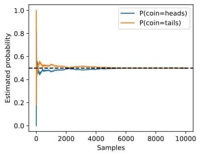
As n → ∞, estimates → true probabilities

Error decreases at rate 1/√n (Central Limit TheoremA fundamental theorem stating that the distribution of sample means approaches a normal distribution as sample size increases.)

Interactive Coin Toss Simulator

Test Your Understanding

Formal Probability Theory

Mathematical foundations

Key Concepts:

Sample SpaceThe set S of all possible outcomes of a random experiment. (S): All possible outcomes
EventA subset of the sample space representing outcomes of interest. (A): Subset of sample space
Probability FunctionA function P that maps events to real numbers between 0 and 1.: P: A → [0,1]

Example: Rolling a die

S = {1, 2, 3, 4, 5, 6}
Event "odd number" = {1, 3, 5}
P(odd) = 3/6 = 0.5

Probability Axioms (Kolmogorov)

Three Fundamental Axioms:

1. Non-negativity: P(A) ≥ 0

2. Normalization: P(S) = 1

3. Additivity: For disjoint events A₁, A₂, ...

$$P\left(\bigcup_{i=1}^{\infty} A_i\right) = \sum_{i=1}^{\infty} P(A_i)$$

All probability theory follows from these three axioms!

Random Variables

Mapping outcomes to values

A random variableA function that maps outcomes from a sample space to numerical values. X maps sample space to values

Types:

Discrete: Countable values (dice, coins)
Continuous: Uncountable values (height, weight)

Notation:

P(X = x): Probability that X takes value x
P(X): Distribution of X
P(a ≤ X ≤ b): Probability X is in range [a,b]

Probability Distributions

Multiple Random Variables

Joint and conditional probabilities

Joint Probability:

P(A = a, B = b) - probability of both events

Key Property:

$$P(A=a, B=b) \leq P(A=a) \text{ and } P(A=a, B=b) \leq P(B=b)$$

Marginalization:

$$P(A=a) = \sum_b P(A=a, B=b)$$

Conditional Probability

Probability given additional information

Definition:

$$P(B=b \mid A=a) = \frac{P(A=a, B=b)}{P(A=a)}$$

Interpretation:

Probability of B=b, given that we know A=a occurred

Conditioning restricts the sample space and renormalizes probabilities

Bayes' Theorem

Reversing conditional probabilities

$$P(A \mid B) = \frac{P(B \mid A) P(A)}{P(B)}$$

Components:

P(A): Prior probability
P(B|A): Likelihood
P(A|B): Posterior probability
P(B): Evidence (normalizing constant)

"Posterior = Prior × Likelihood / Evidence"

Independence

When events don't affect each other

Definition: A and B are independent (A ⊥ B) if:

$$P(A \mid B) = P(A)$$

Equivalent condition:

$$P(A, B) = P(A) \cdot P(B)$$

Conditional Independence:

A ⊥ B | C if P(A, B | C) = P(A | C) · P(B | C)

Test Your Understanding

Example: Medical Testing

Applying Bayes' theorem to HIV testing

Test characteristics:

Sensitivity: P(Positive | HIV) = 1.0
False positive rate: P(Positive | Healthy) = 0.01
Disease prevalence: P(HIV) = 0.0015

Question: If test is positive, what's P(HIV)?

Calculating with Bayes' Theorem

Step 1: Calculate P(Positive)

$$P(Pos) = P(Pos|HIV)P(HIV) + P(Pos|Healthy)P(Healthy)$$

$$= 1.0 \times 0.0015 + 0.01 \times 0.9985 = 0.011485$$

Step 2: Apply Bayes' theorem

$$P(HIV|Pos) = \frac{P(Pos|HIV)P(HIV)}{P(Pos)}$$

$$= \frac{1.0 \times 0.0015}{0.011485} = 0.1306$$

Only 13.06% chance of HIV despite positive test!

Second Test Analysis

Improving confidence with multiple tests

Second test (less accurate):

P(Pos₂ | HIV) = 0.98
P(Pos₂ | Healthy) = 0.03

Both tests positive:

P(HIV | Pos₁, Pos₂) = 0.8307

Second test dramatically increases confidence to 83.07%!

Interactive Bayes Calculator

Explore how prior and test accuracy affect posterior

Expectations

Average values of random variables

Definition:

$$E[X] = \sum_{x} x \cdot P(X = x)$$

Investment Example:

50% chance: 0× return (total loss)
40% chance: 2× return
10% chance: 10× return

E[Return] = 0.5×0 + 0.4×2 + 0.1×10 = 1.8×

Variance and Standard Deviation

Measuring spread and risk

Variance:

$$\text{Var}[X] = E[(X - E[X])^2] = E[X^2] - E[X]^2$$

Standard Deviation:

$$\sigma = \sqrt{\text{Var}[X]}$$

Variance quantifies uncertainty and risk in predictions

Properties of Expectation

Linearity:

E[aX + bY] = aE[X] + bE[Y]

Function of Random Variable:

$$E[f(X)] = \sum_x f(x) \cdot P(X = x)$$

For vectors:

Covariance matrix: Σ = E[(X - μ)(X - μ)ᵀ]

Test Your Understanding

Types of Uncertainty

Aleatoric vs Epistemic

Aleatoric Uncertainty:

Inherent randomness in the problem
Cannot be reduced with more data
Example: Coin toss outcomes

Epistemic Uncertainty:

Uncertainty about model parameters
Can be reduced with more data
Example: Estimating coin fairness

Convergence and Sample Complexity

How fast do we learn?

Rate of convergence: 1/√n

Implications:

10 → 1000 samples: 10× reduction in uncertainty
1000 → 2000 samples: Only 1.41× reduction

Diminishing returns: Easy gains initially, then harder improvements

Key Takeaways

1. Foundation of ML: Probability quantifies uncertainty

2. Bayes' Theorem: Update beliefs with evidence

3. Expectations: Summarize distributions

4. Convergence: More data → Better estimates

These concepts underpin all of machine learning!

Final Test

Calculus for Deep Learning

Chapter 2.4: Fundamentals of Optimization

Understanding rates of change and gradients

Why Calculus for Deep Learning?

Calculus is the mathematical foundation of optimization

Derivatives: How functions change
Gradients: Direction of steepest ascent
Chain rule: Backpropagation algorithm
Optimization: Minimize loss functions

Every parameter update in deep learning uses calculus!

Archimedes' Method

Finding the area of a circle through limits

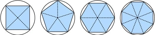
As n → ∞, polygon area → πr²

This limiting procedureA mathematical technique where we examine what happens to a quantity as a parameter approaches a specific value, often infinity or zero. is at the heart of calculus

Test Your Understanding

Derivatives and Differentiation

Understanding rates of change

A derivativeThe rate of change of a function with respect to its input. It tells us how much the output changes when we make a small change to the input. measures how a function changes

Formal Definition:

$$f'(x) = \lim_{h \rightarrow 0} \frac{f(x+h) - f(x)}{h}$$

The derivative tells us the slope at any point!

Numerical Example

Let's compute a derivative numerically

For f(x) = 3x² - 4x at x = 1:

def f(x):
    return 3 * x**2 - 4 * x

# Numerical approximation
x = 1
for h in [0.1, 0.01, 0.001, 0.0001]:
    derivative = (f(x + h) - f(x)) / h
    print(f"h={h}: f'(1) ≈ {derivative:.5f}")

h=0.1:    f'(1) ≈ 2.30000
h=0.01:   f'(1) ≈ 2.03000
h=0.001:  f'(1) ≈ 2.00300
h=0.0001: f'(1) ≈ 2.00030

As h → 0, f'(1) → 2

Common Derivative Rules

Essential formulas for deep learning

Function	Derivative
$$C$$ (constant)	$$0$$
$$x^n$$	$$nx^{n-1}$$
$$e^x$$	$$e^x$$
$$\ln(x)$$	$$\frac{1}{x}$$
$$\sin(x)$$	$$\cos(x)$$

Composition Rules

Combining derivatives

Sum Rule:

$$\frac{d}{dx}[f(x) + g(x)] = f'(x) + g'(x)$$

Product Rule:

$$\frac{d}{dx}[f(x) \cdot g(x)] = f(x) \cdot g'(x) + g(x) \cdot f'(x)$$

Chain Rule:

$$\frac{d}{dx}[f(g(x))] = f'(g(x)) \cdot g'(x)$$

Derivative Visualization

Test Your Understanding

Visualizing Derivatives

Tangent lines and slopes

The derivative at a point equals the slope of the tangent lineA line that touches a curve at exactly one point and has the same slope as the curve at that point.

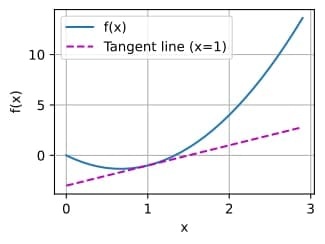
Interactive Tangent Line

Move your mouse to see how the derivative changes

Notice how the slope changes as you move along the curve!

Critical Points

Where derivatives equal zero

When f'(x) = 0:

Local minimum: Valley point
Local maximum: Peak point
Inflection point: Change in curvature

Finding where f'(x) = 0 is key to optimization!

Test Your Understanding

Partial Derivatives

Derivatives for multivariate functions

For f(x, y), we can take derivatives with respect to each variable:

$$\frac{\partial f}{\partial x} = \lim_{h \to 0} \frac{f(x+h, y) - f(x, y)}{h}$$

$$\frac{\partial f}{\partial y} = \lim_{h \to 0} \frac{f(x, y+h) - f(x, y)}{h}$$

Treat other variables as constants!

Example: Partial Derivatives

Let f(x, y) = 3x²y + 5e^y

Partial with respect to x:

$$\frac{\partial f}{\partial x} = 6xy$$

(treat y as constant)

Partial with respect to y:

$$\frac{\partial f}{\partial y} = 3x² + 5e^y$$

(treat x as constant)

The Gradient Vector

Combining all partial derivatives

The gradientA vector containing all partial derivatives of a function. It points in the direction of steepest increase. is a vector of partial derivatives:

$$\nabla f = \begin{bmatrix} \frac{\partial f}{\partial x_1} \\ \frac{\partial f}{\partial x_2} \\ \vdots \\ \frac{\partial f}{\partial x_n} \end{bmatrix}$$

The gradient points in the direction of steepest ascent!

Gradient in Deep Learning

Loss function optimization

For a loss function L(w₁, w₂, ..., wₙ):

$$\nabla_w L = \begin{bmatrix} \frac{\partial L}{\partial w_1} \\ \frac{\partial L}{\partial w_2} \\ \vdots \\ \frac{\partial L}{\partial w_n} \end{bmatrix}$$

Gradient Descent Update:

$$w_{new} = w_{old} - \alpha \cdot \nabla_w L$$

where α is the learning rate

Partial Derivatives Visualization

Test Your Understanding

The Chain Rule

Differentiating composite functions

For nested functions y = f(g(x)):

$$\frac{dy}{dx} = \frac{dy}{du} \cdot \frac{du}{dx}$$

where u = g(x)

The chain rule is the foundation of backpropagation!

Chain Rule Example

Let y = (3x² + 2x)⁵

Step 1: Identify inner and outer functions

Inner: u = 3x² + 2x
Outer: y = u⁵

Step 2: Find derivatives

dy/du = 5u⁴
du/dx = 6x + 2

Step 3: Apply chain rule

dy/dx = 5(3x² + 2x)⁴ · (6x + 2)

Multivariate Chain Rule

For functions of multiple variables

If y = f(u₁, u₂, ..., uₘ) and each uᵢ = gᵢ(x₁, x₂, ..., xₙ):

$$\frac{\partial y}{\partial x_i} = \sum_{j=1}^{m} \frac{\partial y}{\partial u_j} \cdot \frac{\partial u_j}{\partial x_i}$$

Matrix form:

$$\nabla_x y = J^T \cdot \nabla_u y$$

where J is the Jacobian matrix

Chain Rule Visualization

Gradients flow backwards through the computation graph!

Backpropagation

Chain rule in neural networks

For a simple network: Input → Hidden → Output → Loss

$$\frac{\partial L}{\partial W_1} = \frac{\partial L}{\partial z_2} \cdot \frac{\partial z_2}{\partial a_1} \cdot \frac{\partial a_1}{\partial z_1} \cdot \frac{\partial z_1}{\partial W_1}$$

L: Loss function
z: Pre-activation values
a: Activation values
W: Weight matrices

Test Your Understanding

Gradient Descent in Action

Optimizing a simple loss function

Each step moves in the negative gradient direction!

Learning Rate Impact

Choosing the right step size

Too small: Slow convergence
Too large: Overshooting, divergence
Just right: Efficient convergence

Update rule:

$$w_{t+1} = w_t - \alpha \cdot \nabla L(w_t)$$

α is the learning rate

Computing Gradients in PyTorch

Automatic differentiation in practice

import torch

# Define variables with gradient tracking
x = torch.tensor([2.0], requires_grad=True)
y = torch.tensor([3.0], requires_grad=True)

# Define function: z = x² + xy + y²
z = x**2 + x*y + y**2

# Compute gradients
z.backward()

print(f"∂z/∂x = {x.grad.item()}")  # 7.0
print(f"∂z/∂y = {y.grad.item()}")  # 8.0

PyTorch automatically applies the chain rule!

Neural Network Gradients

Backpropagation example

import torch
import torch.nn as nn

# Simple network
model = nn.Sequential(
    nn.Linear(10, 5),
    nn.ReLU(),
    nn.Linear(5, 1)
)

# Forward pass
x = torch.randn(32, 10)  # Batch of 32 samples
y_true = torch.randn(32, 1)
y_pred = model(x)

# Compute loss
loss = nn.MSELoss()(y_pred, y_true)

# Backward pass (compute gradients)
loss.backward()

# Access gradients
for name, param in model.named_parameters():
    print(f"{name}: gradient shape = {param.grad.shape}")

Key Takeaways

1. Derivatives measure change

Essential for understanding how parameters affect loss

2. Gradients point uphill

We move opposite to minimize loss

3. Chain rule enables backpropagation

Gradients flow backward through networks

4. Automatic differentiation

Frameworks handle the math for us

Final Test

Automatic Differentiation

Computing gradients automatically

Manual derivative calculation is:

Tedious and error-prone
Complex for large models
Difficult to maintain

Autograd makes deep learning practical!

What is Automatic Differentiation?

Automatic differentiationA technique to evaluate derivatives of functions specified by computer programs with machine precision (autograd):

Computes exact derivatives (not numerical approximations)
Builds computational graphsA directed graph where nodes represent operations and edges represent data flow dynamically
Applies chain rule automatically

Historical Context:

First references: 1960s (Wengert, 1964)
Modern backpropagation: 1980s (Speelpenning, 1980)
Framework integration: 2010s

Computational Graphs

How autograd tracks computations

Each operation creates a node in the graph!

Backpropagation Algorithm

Applying chain rule backwards through the graph

Forward pass: Compute outputs and build graph
Backward pass: Compute gradients using chain rule
Update: Use gradients to update parameters

$$\frac{\partial L}{\partial w} = \frac{\partial L}{\partial y} \cdot \frac{\partial y}{\partial w}$$

Chain rule applied recursively

Test Your Understanding

A Simple Function

Computing gradients in PyTorch

Let's differentiate: $$y = 2\mathbf{x}^T\mathbf{x}$$

with respect to vector $\mathbf{x}$

import torch

# Create tensor and enable gradient tracking
x = torch.arange(4.0, requires_grad=True)
print(x)  # tensor([0., 1., 2., 3.], requires_grad=True)
print(x.grad)  # None (no gradient computed yet)

requires_grad=True tells PyTorch to track operations!

Computing the Gradient

Forward pass and backward pass

# Forward pass: compute y
y = 2 * torch.dot(x, x)
print(y)  # tensor(28., grad_fn=)

# Backward pass: compute gradients
y.backward()

# Access the gradient
print(x.grad)  # tensor([0., 4., 8., 12.])

Verification:

$$\frac{\partial y}{\partial \mathbf{x}} = \frac{\partial}{\partial \mathbf{x}}(2\mathbf{x}^T\mathbf{x}) = 4\mathbf{x}$$

At x = [0,1,2,3]: gradient = [0,4,8,12] ✓

Gradient Accumulation

PyTorch accumulates gradients by default

# Compute gradient of sum
x.grad.zero_()  # Reset gradient to zero
y = x.sum()
y.backward()
print(x.grad)  # tensor([1., 1., 1., 1.])

# Without resetting - gradients accumulate!
y = x.sum()
y.backward()
print(x.grad)  # tensor([2., 2., 2., 2.]) - accumulated!

Always call grad.zero_() before computing new gradients!

Gradient Computation Visualization

Watch how gradients flow backward through the graph

Test Your Understanding

Backward for Non-Scalar Variables

Handling vector and matrix outputs

When output is not scalar, we need the JacobianA matrix of all first-order partial derivatives of a vector-valued function:

$$J = \begin{bmatrix} \frac{\partial y_1}{\partial x_1} & \cdots & \frac{\partial y_1}{\partial x_n} \\ \vdots & \ddots & \vdots \\ \frac{\partial y_m}{\partial x_1} & \cdots & \frac{\partial y_m}{\partial x_n} \end{bmatrix}$$

PyTorch requires scalar output or gradient argument!

Vector Gradients in Practice

Using the gradient argument

x.grad.zero_()
y = x * x  # Element-wise square, output is vector

# Method 1: Provide gradient vector
y.backward(gradient=torch.ones(len(y)))
print(x.grad)  # tensor([0., 2., 4., 6.])

# Method 2: Sum to scalar (more common)
x.grad.zero_()
y = x * x
y.sum().backward()  # Same result!
print(x.grad)  # tensor([0., 2., 4., 6.])

The gradient argument computes: $\mathbf{v}^T \cdot J$

Why Sum for Loss Functions?

Batched gradient computation

In deep learning, we often have:

Loss computed per example
Batch of N examples
Need single gradient for parameters

# Typical pattern in training
batch_losses = model(batch_inputs)  # Shape: [batch_size]
total_loss = batch_losses.mean()     # Reduce to scalar
total_loss.backward()                # Compute gradients

Detaching Computation

Controlling gradient flow

Sometimes we need to stop gradients:

Freeze certain parameters
Create non-trainable features
Implement special algorithms

detach() breaks the computational graph!

Detach Example

Breaking gradient flow selectively

x.grad.zero_()
y = x * x
u = y.detach()  # u has same value as y, but no gradient
z = u * x       # z = x³ but gradient treats u as constant

z.sum().backward()
print(x.grad == u)  # True - gradient is u, not 3x²!

# Compare with normal computation
x.grad.zero_()
z_normal = x * x * x
z_normal.sum().backward()
print(x.grad)  # This would be 3x²

With detach: $\frac{\partial z}{\partial x} = u = x^2$

Without: $\frac{\partial z}{\partial x} = 3x^2$

Practical Use Cases

When to use detach()

1. Feature extraction:

features = pretrained_model(x).detach()
output = custom_head(features)  # Only train head

2. Stop gradient in GANs:

fake = generator(noise)
disc_fake = discriminator(fake.detach())  # Don't update G

3. Reinforcement learning:

target_value = reward + gamma * next_value.detach()

Gradient Flow Visualization

Red edges show where gradients are blocked

Gradients and Python Control Flow

Dynamic computational graphs

Autograd handles arbitrary Python code:

Conditionals (if/else)
Loops (for/while)
Function calls
Recursion

Graph is built dynamically during execution!

Control Flow Example

Gradients through conditions and loops

def f(a):
    b = a * 2
    while b.norm() < 1000:
        b = b * 2
    if b.sum() > 0:
        c = b
    else:
        c = 100 * b
    return c

# Different inputs create different graphs!
a = torch.randn(size=(), requires_grad=True)
d = f(a)
d.backward()

# Gradient still computed correctly
print(a.grad)  # Works despite complex control flow!

Each execution may create a different graph!

Dynamic vs Static Graphs

PyTorch's approach to autograd

Dynamic Graphs (PyTorch):

Built during forward pass
Can change every iteration
Natural Python control flow
Easy debugging

Use cases:

Variable-length sequences (NLP)
Tree/graph neural networks
Conditional computation

Gradient Verification

Checking autograd correctness

# Function f is linear with piecewise scale
a = torch.randn(size=(), requires_grad=True)
d = f(a)
d.backward()

# Verify gradient matches theory
# Since f is piecewise linear: f(a) = scale * a
# Therefore: df/da = scale
scale = (d / a).item()
expected_grad = scale

print(f"Computed gradient: {a.grad.item()}")
print(f"Expected gradient: {expected_grad}")
print(f"Match: {torch.allclose(a.grad, torch.tensor(expected_grad))}")

Test Your Understanding

Automatic Differentiation Best Practices

1. Memory Management:

Use torch.no_grad() for inference
Detach intermediate results when needed
Clear gradients with zero_()

2. Debugging:

Use retain_graph=True sparingly
Check grad_fn attribute
Verify gradient shapes

3. Performance:

Avoid unnecessary gradient tracking
Use in-place operations carefully
Profile gradient computation

Common Pitfalls

Avoiding autograd mistakes

❌ Forgetting to zero gradients:

for epoch in range(100):
    loss = model(x)
    loss.backward()  # Gradients accumulate!

✓ Correct approach:

for epoch in range(100):
    optimizer.zero_grad()  # Reset gradients
    loss = model(x)
    loss.backward()

❌ Modifying tensors with gradients:

x = torch.randn(3, requires_grad=True)
x[0] = 1  # Error! Can't modify tensor with gradients

Higher-Order Derivatives

Computing gradients of gradients

# First derivative
x = torch.tensor([2.0], requires_grad=True)
y = x ** 3  # y = x³

# First derivative: dy/dx = 3x²
grad1 = torch.autograd.grad(y, x, create_graph=True)[0]
print(f"First derivative at x=2: {grad1}")  # 12

# Second derivative: d²y/dx² = 6x
grad2 = torch.autograd.grad(grad1, x)[0]
print(f"Second derivative at x=2: {grad2}")  # 12

Use create_graph=True to compute higher-order derivatives!

Key Takeaways

1. Automatic differentiation is exact

Not numerical approximation

2. Computational graphs are dynamic

Built during forward pass

3. Gradients accumulate by default

Remember to zero them!

4. Control flow is handled naturally

Write normal Python code